Millimeter Wave Experimental Field Setup
POSTED ON SEPTEMBER 15, 2022 BY TMYTEK
Abstract
A hundred meters millimeter wave transmission is demonstrated by TMYTEK’s rapid prototyping platform. Academics and businesses have been working hard to create new innovation and further research on the millimeter wave experiments such as 5G millimeter wave commercialisation approaches. Measuring over-the-air transmission performance is one of the essential experiments to get to know how millimeter wave works in the real environment to assist operators evaluate the number of base stations that are required for any specific area. The experiment expedites the development of beamforming and beam tracking algorithms in addition to making base station construction simpler for telecom operators. Conducting related research and data analysis is crucial for the millimeter wave experimental sector.
With the 256 QAM modulation scheme, we will demonstrate a 100-meter millimeter wave communication while preserving an excellent EVM performance. Learn about the function of each communication component and the theory behind them to enhance the performance while simultaneously attempting to understand the impact of the demonstration.
Introduction
A suitable millimeter wave experimental field must be identified and prepared in order to conduct research on a number of 5G FR2 technologies, including beamforming, beam tracking, and, in particular, the millimeter wave propagation characteristics. Establishing a professional experimental field might be difficult for researchers, however TMYTEK has designed a quick mmWave prototype platform that is capable of making the construction of the field setup easier. In this article, we'll examine the platform's architecture, evaluate each component's dynamic range and link budget, and adjust the RF parameters to increase the transmission distance from 20 to 100 meters and at the same time reduce the amplitude of the error vector (EVM).
Platform Architecture
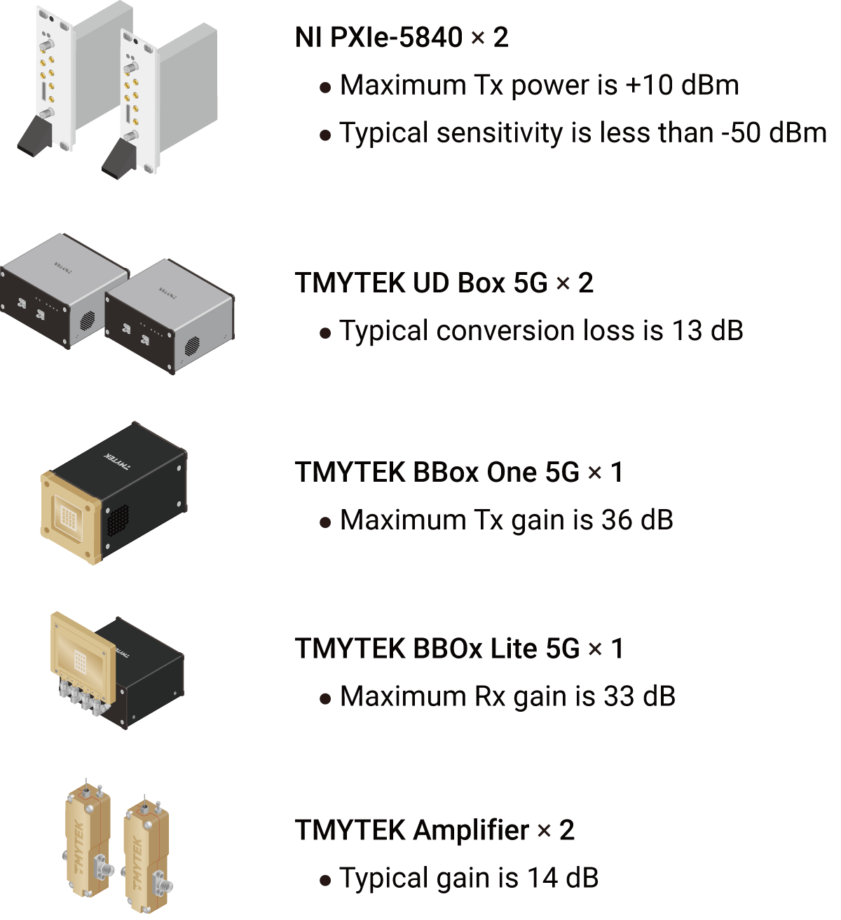
As shown in Figure 1, the baseband, up-down converter, and beamformer are the three main components of a typical millimeter wave communication system. With NI’ s PXIe-5840 VST serv- ing as the baseband, TMYTEK’s UD Box 5G serving as the frequency converter, TMYTEK’s BBox 5G serv- ing as the beamformer along withTMYTEK’ s amplifiers for link budget optimization, the real-world implementation is depicted in Figure 2.
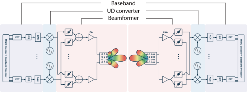 Figure 1: Millimeter Wave System Architecture
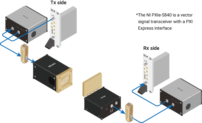 Figure 2: Platform of TMYTEK’s Millimeter Wave Communication System
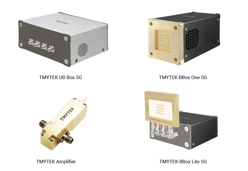 Figure 3 : TMYTEK products that are typically used in the TMYTEK mmWave Communication Platform
To achieve a transmission distance of 100 meters, the system link budget and the path attenua- tion are two crucial factors. The system link budget and the dynamic ranges of each component are discussed in the following sections.
System Link Budget
Figure 4 shows the link budget for the entire system and highlights the gain or loss that each component contributed.
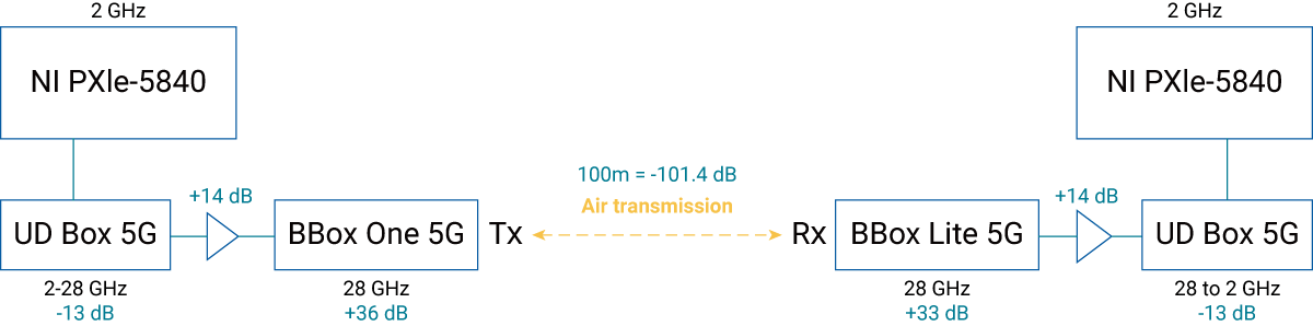 Figure 4: Link Budget Architecture
*The maximum distance limited by this communication prototype is a critical concern about this experiment.
The equipment used and the gain/loss contributions are listed below.
Link budget of free space loss =
Tx transmitter power - Rx received or sensitivity power +
Total Tx gain + Total Rx gain - Total Tx loss - Total Rx loss
LFS = PTx-PRx+(GAmp+GOne)+(GLite+GAmp) -(LUD+LTx)-(LUD+ LRx)
- where
- LFS = Free-space loss (dB)
- PTx = NI-5840 transmitter power output (dBm)
- PRx = NI-5840 received power or received sensitivity (dBm)
- GAmp = Power amplifier gain (dB)
- GOne = BBox One 5G transmitter gain (dB)
- GLite = BBox Lite 5G receiver gain (dB)
- LUD = UD Box 5G conversion loss (dB)
- LTx = Total cable loss from transmitter side (dB)
- LRx = Total cable loss from receiver side (dB)
The following formula is used to calculate free-space attenuation vs distance based on operating frequency. Table 1 shows the attenuation for various distances.
L = 20 log [ 4πd/λ]
- where
- L= free space transmission loss (dB)
- d= distance
- λ= wavelength
 Table 1: Free Space Path Loss at 28GHz
The margin for free space loss is around 102 dB to reach the 100 meters transmission. The fol- lowing stage entails examining the dynamic range in order to determine the proper input power for each device and to determine how to stay within the acceptable loss level by modifying the gain within this link.
Dynamic Range of Components
UD Box 5G's dynamic range
The dynamic range of the UD Box 5G in both up- and down-conversion is
depicted by the bathtub curves in Figure 5. The X-axis represents the
input power, while the Y-axis represents the mea- sured signal quality
(EVM) at the output. While the input power is high and the output
surpasses the linear region of the UD Box 5G, the EVM is poor. On the
other hand, when the input signal is weak, the performance of the EVM
is determined by the noise floor.
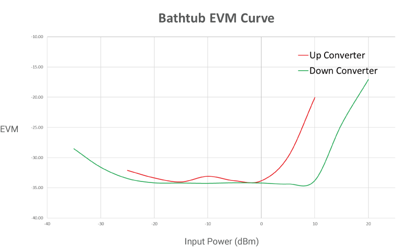 Figure 5: Bathtub EVM curve (IF = 2GHz , RF = 28GHz)
BBox 5G's dynamic range
The characteristic performances for Gain, P1dB, and Noise Figure (NF)
are the three most crucial parameters in beamforming that can affect
the transmission distance. Based on the specifica- tion mentioned in
Table 2, BBox Lite 5G is set up as a receiver with the appropriate NF to
increase the sensitivity while BBox One 5G is configured as a transmitter
with high gain to achieve the best EIRP.
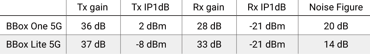 Table 2: Specifications for BBox at 28GHz
Procedure
Keysight’ s signal generator (M9384B) and signal analyzer (N9042B) were used in place of the NI-5840 and UD Box 5G set because they can generate and measure directly at 28 GHz. This set of setup is called the control group (CG) and is used as the baseline for comparison with the other comparison groups test results, which can be seen in the later sections. And the experimental group (EG) setup is shown in Figure 2. In the following experiments, the experimental group (EG) and the control group (CG) will be tested in the same environment, and the results will be com- pared and analyzed.
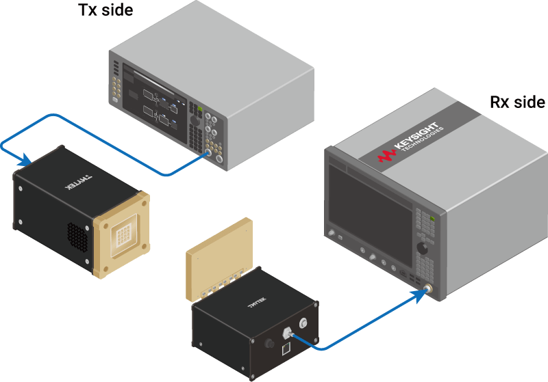 Figure 6: Transmitter and receiver setup for control group
Both indoor and outdoor millimeter wave propagation will be investigated. We can determine how different circumstances affect the transmission by comparing the theoretical link budget with the actual signal strength. To achieve the greatest transmission distances, we determine the power level that best matches the dynamic range of each device.
In open space, higher Tx power travels further. As seen in Figure 7, in order to attain the highest EIRP (38 dBm), the baseband's output power must be reduced to mitigate the nonlinearity effect of the amplifiers in BBox.
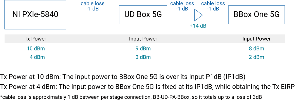 Figure 7 : Maximum EIRP (Equivalent Isotropically Radiated Power) calculation
In order to match the EVM bathtub on the receiver side and compensate for the conversion loss that the UD Box 5G has introduced, a 14 dB amplifier was added in order to increase the power received by the BBox Lite 5G by 33 dBm. This ensures the demodulation performance maintains an excellent EVM.
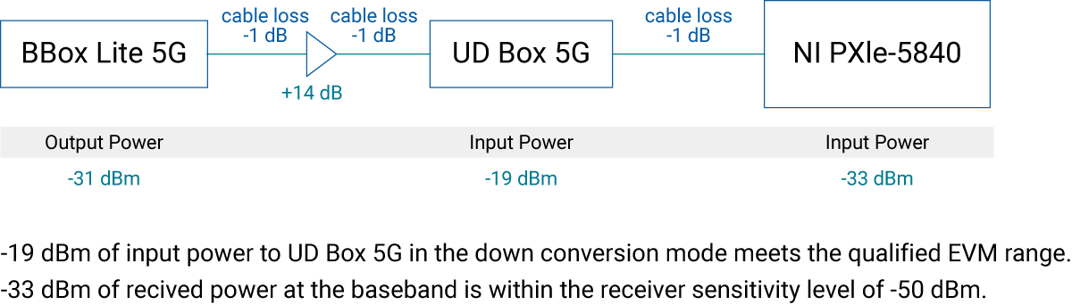 Figure 8 : Receiver link budget at a distance of 100 meters
Figure 9 illustrates how the system could potentially overcome 116 dB of free space loss to reach 500 meters of communication transmission. This is to investigate how much farther it is possible to go, while maintaining the received baseband power within its sensitivity specifica- tions as well as the EVM quality of the UDBox.
Can the system transmit farther? A proposal using MIMO technology is considered. With the use of multiple BBox One 5G to increase the total output power, consequently, the transmission dis- tance can be increased. As the following table suggests, two BBox One 5G doubles the total output power (+3 dB), four BBox One 5G would add 6 dB more output power and so on, in other words, the system could achieve longer transmission distance in theory.
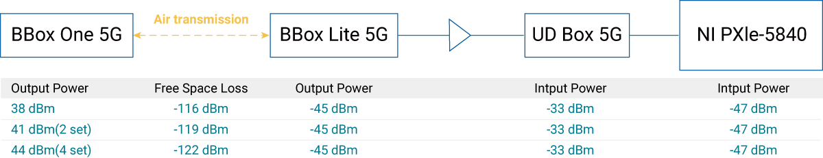 Figure 9 : Possible calculation for MIMO or longer distance transmission
With the following 5G NR FR2 waveform, we examine the indoor transmission distances of 20, 30, 50, and 60 meters:
- 5G NR FR2 waveform setting conditions:
- 28 GHz frequency
- 100 MHz bandwidth
- 120 kHz subcarrier
- 256 QAM
Indoor testing distances : 20 m, 30 m, 50 m and 60 m
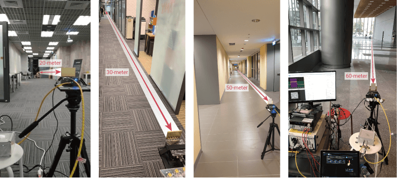 Figure 10: Indoor Field Test Conditions
The effect of Tx power and amplifiers on the transmission distance is depicted in Table 3. Please be aware that the control group (CG) conducted in these studies in the mmWave bands elimi- nates the influence of the UD Box 5G, as well as Tx power and Rx sensitivity. This is a great opportu- nity to assess the effects of the link budget and the UD Box 5G.
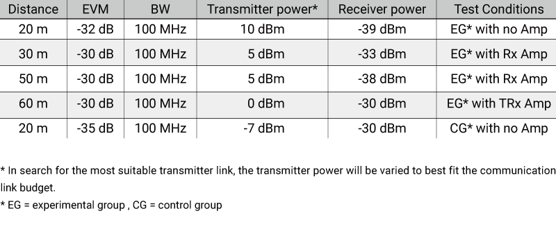 Table 3: Indoor Test Data
Outdoor testing distances: 60 m, 80 m, 100 m
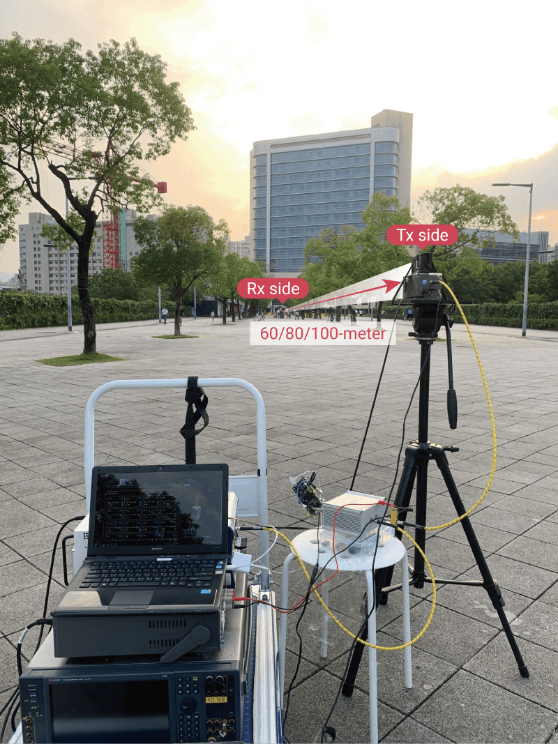 Figure 11: Outdoor Field Test Conditions
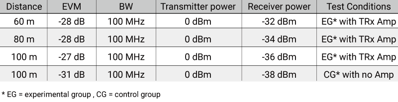 Table 4: Outdoor Test Data
Because of multipath superimposition, indoor signals always outperform outdoor signals with better EVM performances for a given transmission distance. By contrasting the theoretical link budget with the measured data, further evaluation can be done from these insights.
LFS = PTx-PRx+(GAmp+GOne)+(GLite+GAmp) -(LUD + LTx)-(LUD+LRx)
The following equation can be obtained for the calculation of the received power by rearranging the equation.
PRx=PTx-LUD+GAmp+GOne-LTx-LFS+GLite+GAmp-LUD-LRx
Below is a theoretical calculation of the received power at a distance of 100 meters. 0dBm(PTx)-13dB(LUD)+14dB(GAmp)+36dB(GOne)-3dB(LTx)-101.4dB(LFS)+33dB(GLite)+14dB (GAmp)-13dB(LUD)-3dB (LRx) equals -36.4 dBm (PRx)
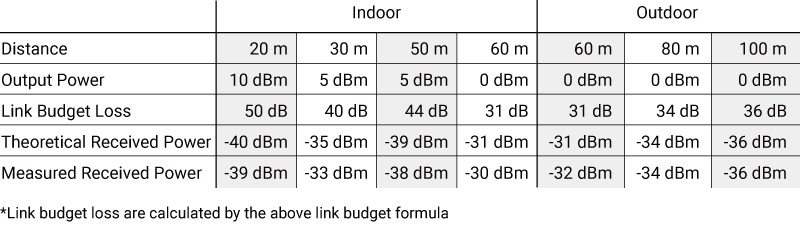 Table 5: Comparison of the theoretical and the measured values of the received power
Measurements are taken and the environment is built as shown above for this field setup. This type of field setup is the simplest, and can be expanded in the future to include longer distances and MIMO field experiments. This setup can be used to reach a number of different technology research and applications.
Summary
Building an actual millimeter wave experimental field, in the opinion of TMYTEK, will help with research such as beamforming algorithms, physical channel detecting characteristics, and millimeter wave commercialization. This application note for a millimeter wave field setup is made simple and quick for researchers to construct and in particular to determine the link budget based on the power dynamic range of the devices used within the communication link as well as the equipment's performance limitations. Furthermore, it is worth noting that the multipath effects that have caused the indoor experiments to have higher signal quality than the outdoor experiments. Another important area of research in the pre-commercial stage is the collection of data on channel parameters. These data will help telecommunication providers to deploy base stations more efficiently.
Download Application Note: Millimeter Wave Experimental Field Setup